Monte Carlo methods for synthetic data generation with LLMs

At Sphinx, we work in domains where high-quality public data is scarce. To bridge that gap, we turn to LLMs as engines for generating synthetic data.

This approach, while powerful, introduces challenges, chief among them the inherent biases baked into LLM inference. As a simple example, consider asking GPT 5-nano to generate a uniformly random number between 0 and 100. Even at high temperatures, which should encourage randomness, models are optimized to output modes, not to be creatively random:

For random numbers, the obvious answer is to use traditional sources of randomness to generate a fair sample. For more complex data types it may not be possible to sample distributions directly.

Luckily, LLMs do provide us with a group of tools which we can use to improve sampling through classical methods. We explore a method inspired by Markov Chain – Monte Carlo (MCMC) methods and Metropolis-Hastings sampling. These methods help when a distribution over a domain 𝒟 is hard to sample, but we do have access to a function proportional to the distribution of interest. In the case of LLM-driven sampling of a uniform distribution 𝒟, this simply amounts to an indicator function

𝑔(𝑥) = [[𝑥 ∈ 𝒟]]

In many cases, 𝑔 can be defined by simple rules, an LLM, or a combination of both. For example, consider sampling from the space of restaurant reviews – an LLM can easily verify if a string is a plausible review even if it may have issues with generating unbiased samples.

The second ingredient needed for Metropolis-Hastings sampling is a proposal function which, given a point 𝑥 ∈ 𝒟, gives a distribution 𝑞(𝑧|𝑥) over 𝒟. This too can be implemented via LLM, by prompting a model to generate new examples similar, but not identical to, an existing example.

The Metropolis-Hastings algorithm then collapses to the following steps:

1. First, draw a (almost certainly biased) sample 𝑥 ∈ 𝒟 using an LLM to suggest an example
2. Then, in a loop:
   • Draw 𝑧 ∼ 𝑞(⋅ | 𝑥 )
   • If 𝑔(𝑧), accept the new sample with probability 𝑞(𝑧|𝑥)/𝑞(𝑥|𝑧) and set 𝑥 ← 𝑧. In the case where 𝑞 is symmetric in its arguments, the acceptance probability is 1 if 𝑔(𝑧).
   • Otherwise, we reject the sample and leave 𝑥 ← 𝑥
3. At the completion of 𝑁 of iterations of the loop, output 𝑥 as a sample from 𝒟

Assumptions for Metropolis-Hastings to Generate Unbiased Samples

There are several assumptions we need on 𝑞 to meet to guarantee that in the limit 𝑁→ ∞, 𝑥 is distributed uniformly across 𝒟:

1. Irreducibility: For any states 𝑥′, 𝑥 ∈ 𝒟, there should exist some way for the algorithm to sample 𝑥′ starting from 𝑥. This is almost certainly true for an LLM, there should be nonzero probability on almost all tokens and therefore some path for 𝑥′ to be generated by 𝑞
2. Aperiodicity: That there are no deterministic cycles induced by the sampling. This is mitigated by the fact that not all 𝑧 are accepted, giving a nonzero probability of 𝑥 not changing in a given step. By assigning a nonzero temperature to the LLM used to determine 𝑔(𝑥), this is guaranteed.
3. Detailed Balance: We need to be able to compute 𝑞(𝑥′|𝑥)/𝑞(𝑥|𝑥′), to ensure we are equally likely to sample 𝑥′ starting from 𝑥, and vice-versa. Detail balance is a challenge because 𝑞 is not easily expressible in closed form. A future exercise could be computing this directly from log-probabilities emitted by the LLM, but we opt for a simpler approach:
   • Sample several observed suggestions of 𝑥 → 𝑥′ by running the algorithm with a 100% acceptance rate
   • Construct a dataset of triplets (𝑥, 𝑥′, F) and (𝑥′, 𝑥, R) to train a model to predict the third binary coordinate (whether this was an observed “forward” transition or a synthetic “reverse” transition) as a function of the ordered pair of the first two coordinates.
   • This model, up to constant factors, predicts the relative probability that a transition was from 𝑥 to 𝑥′ vs from 𝑥′ to 𝑥.

In practice, we often find that this probability is very close to 1, in which case detailed balance approximately holds without any correction factors.

Evaluating Synthetic Data Generation

Let’s evaluate LLM-driven Metropolis-Hastings on two problems. In both cases, we use GPT 4.1-mini as our LLM of choice. We leverage Sphinx copilot to quickly code the MCMC algorithm above and to explore, visualize, and validate our results.

Points on the Simplex

We want to use AI to generate points in the three-dimensional simplex: 𝑥, 𝑦, 𝑧 > 0, 𝑥 + 𝑦 + 𝑧 < 1

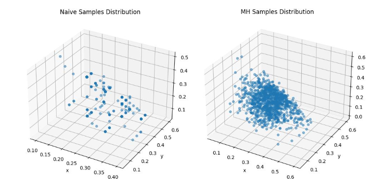
In this case, the proposal function asks the LLM to make up a new point near a given one, and the indicator function deterministically checks the condition above. We note that, like the one-dimensional case, a naive LLM implementation of random sampling 1000 points has extreme concentration on certain values. On the other hand, our Metropolis-Hastings based sampling gets far better coverage of the space.

This is a relatively simple example that confirms our intuition. We next try this method on a harder, realistic problem.

Generating restaurant reviews

We want to generate a diverse set of synthetic restaurant reviews, and benchmark against a real set of around 100,000 Yelp reviews.

For naive generation, we simply ask the LLM to generate a “Yelp review of a restaurant. The review should use real information when possible.”  The proposal function asks the LLM to generate a “different but similar (in theme, content, style, or sentiment) review” to an original review. Lastly, our indicator function simply asks the LLM if a candidate string looks like a valid Yelp review.

First, we verify that detail balance approximately holds. We run 1000 chains of 10 steps each, and collect all generated transitions between reviews. For each before-after pair of reviews, we embed the reviews with OpenAI’s text-embedding-3-small model and find that we can only predict if a transition occurred in the forward or reverse direction with 53% accuracy – this is indicative that our proposal function is approximately symmetric.

To bolster this, we also find that the distribution of changes in embeddings from the proposal function are mean-zero and symmetric, as in the examples below:

With confidence that detail balance holds, we generate 1000 examples using both naive and MCMC based sampling. We visualize the sampled region by embedding all reviews with text-embedding-3-small and projecting with PCA to 2 dimensions. The plots below show a KDE-based contour capturing the support of the distribution generated by each method.

From this initial exploration, we can clearly see that the MCMC-based samples (green) cover more of the space than the naive (orange) samples – but there is still a large area on the left of the plot that is covered by real reviews (blue) that we don’t seem to sample properly.

This was one of the areas where Sphinx copilot really helped. We asked it to sample some data from that region, and in seconds it wrote code to pull the original strings through the whole embedding pipeline and provide some samples, like the following:

“Best Ice Cream in Arizona! The mango margarita sorbet and salted butter carmel are my favorites. They constantly have fun thing new to try. Don’t forget the they have scooped and pre packed pints at whole foods around the valley also.”

Interestingly, almost all Yelp reviews in the uncovered region pertain to ice cream parlors. Simply excluding these with a string filter for “ice cream” in the ground-truth Yelp reviews almost fully solves the problem. For us, this served as a clear cautionary tale that while this method may be helpful, it still relies on robust prompting and a clear understanding of the domain we want to cover – it seemed like the LLM here did not think of ice cream shops as restaurants and therefore did not cover this space.

Excluding these examples, we can now see that MCMC expands the region of coverage of the samples to align closely to the real Yelp data.

To rigorously measure the improvement here, we compute a distributional distance metric between each of the sets of samples and the real Yelp reviews. We train a model to differentiate between the generated samples and real Yelp reviews – we choose a random forest on the embeddings here – and find its log-loss on a held out set.

It can be shown that this log loss is, in the limit of the Bayes-optimal classifier, equivalent to log(2) minus the Jensen-Shannon (JS) divergence of the two underlying distributions. Intuitively, if it is easy to tell which distribution a data point came from the two distributions are quite different from each other and vice-versa.

We thereby estimate the JS-divergence between naive samples and real Yelp reviews to be 0.45 ± 0.003 , and between MCMC samples and real reviews to be 0.43 ± 0.008, showing a statistically significant improvement in sampling.

How are we using insights like these at Sphinx?

Data science, ironically, is a data-deficient field when it comes to AI. Sphinx is using methods like this one to generate robust sets of synthetic data for challenges like representation learning on graphs and understanding realistic business queries.